How To Create Dynamic Charts/Graphs!!!

Watch the Video - How to create Dynamic chart in Excel.

 

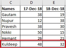
Let say we have the data table as above and we have created a chart below:

Now, I want to update the chart automatically as I update the data table, let say if I add one more name and respective data then my chart should automatically be populated. Below is the updated data:

For that, we need to follow below steps:

Step 1: Create dynamic name ranges for each column. To create dynamic range use below functions

i)   Names = "=OFFSET(Sheet1!$C$2,0,0,COUNTA(Sheet1!$C:$C)-1,1)"

ii)  Date1   = "=OFFSET(Sheet1!$D$2,0,0,COUNTA(Sheet1!$D:$D)-1,1)"

iii) Date2  =  "=OFFSET(Sheet1!$E$2,0,0,COUNTA(Sheet1!$E:$E)-1,1)"

Step 1.1

Goto Name Manager > Click on New > Type your name under Name section and Put below formulas under Refers to section

Step 1.2

Step 2: Goto 'Insert' Tab and create a Column Chart, you chart will be blank

Step 3: Now, Right click on the chart area and click on "Select Data", and click on 'Add' icon under Legend Entries. See below:

Step 3

Step 4: Select or Type your Date from the sheet, e.g., 17-Dec-18 in Series Name and Type =Sheet1!Date1 in Series Values. See below:

Step 4: D1 is your date, Sheet1 is your Sheet name & Date1 is your Name range which we have provided to the range.

Step 5: Click on Edit under Horizontal (Category) Axis Labels and type =Sheet1!Names in Axis Label Range. See below:

Step 5.1

Step 5.2

Step 6: Now click on 'Add' icon under Legend Entries and do the same steps for Date2.

Your Data Source tab will look like below image:

And your chart will look like below image:

---------------------------------------------------------------------------------------------------------------------------------------------------------------

Download the file: Dynamic Chart.xlsx

Thanks for learning, will come soon with new post.